
Gauging the potential of Chrome using the Bass model (part 1)
23 Sep 2008On September 2, 2008, Google launched its browser, Chrome, with great buzz in the geekosphere. I gave it a spin, but stayed with Firefox (old habits die hard), and did not give it more thought until I came across this post where Donn Felker ventures his gut feeling for what the browser market will look like in 2009.
I believe that his forecast, while totally subjective, qualifies as an “expert opinion”, and is essentially correct, and wondered what quantitative analysis methods would add to it - and decided to give it a shot.
The Bass adoption model
Properly representing the introduction of a new product on the market is a classic problem in quantitative modeling. At least two factors make it tricky: there is only limited data available (because it’s a new product), and the underlying model cannot be linear (because it starts from 0, and has a finite growth).
In 1969, Frank Bass proposed a model which is now a classic. It represents adoption as the combination of two factors: innovation and imitation. Innovators are the guys you see in line at the Apple store when a new iGizmo is launched; they have to have it first, regardless of how many people have it already. Imitators are the cautious ones, who will jump on board when enough people are using the product already - the more people already adopted, the more imitation will take place.
In terms of dynamics, innovators determine the early pick-up of the product, and create the initial critical mass of users - and imitators drive the bulk of the growth, going from early adoption to peak.
The mathematical formulation of the model goes like this:
It is a very elegant and lightweight model, which takes only 3 parameters, and is surprisingly good at replicating actual adoption. The Excel model attached provides an illustration of the dynamics of the model, depending on its input parameters, the total population, and the rates of innovation and imitation.
Using the Bass model to determine market potential
Imagine now that you had some data on the early uptake of a new product on the market. How could you use the Bass model to predict its long term adoption?
For the sake of illustration, let’s suppose that your product has been launched in January, and that you have only partial data so far, for March through October.
| Month | Market Share |
|---|---|
| March | 3.43% |
| April | 5.15% |
| May | 7.22% |
| June | 9.68% |
| July | 12.51% |
| August | 15.69% |
| September | 19.14% |
| October | 22.73% |
If you plot this data, you will see that it is fairly close to a straight line, because it is still early in the adoption process, and as a result, it is pretty difficult to guess what the end value will be.
One possible approach is to assume that the introduction follows a Bass curve, and find the 3 parameters for that Bass curve that fit your data as closely as possible. One of the three parameters is the market potential, which can be read directly off the results of the curve fitting process.
I created an Excel spreadsheet which does this automatically using the Solver. I will only outline the general principles I followed here, because going into details would go way beyond the scope of that post.
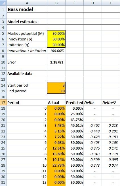
The worksheet sets up side by side the actual historical data and the “theoretical” value of the Bass model. For each period, the square of the difference between the actual and theoretical value is computed; the worse the fit, the higher the number. The overall quality of the fit is measured as the sum of the square differences, so that a perfect fit will result in a zero-sum.
I added a minor feature to accommodate the case where only partial data is available. In our case, the series begins in 3rd period, and ends in 10th, so we will set it to 3 and 10, so as to ignore values outside of that range.
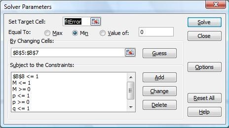
To use the spreadsheet and find the best fit, simply paste your actual data into the orange section labeled “Actual”, select the Solver (which is under the data tab in Excel 2007), and hit “Solve” (The Solver is part of all Excel versions, but may not be installed by default). I set up the solver so that it will “tweak” the 3 arguments of the Bass curve, starting from the initial values, to improve iteratively the sum of the differences. The result will be a best-fit which tries to match the actual curve as closely as possible.
I illustrated below how the process would look like on the illustration data.
Initial setup
Launching the Solver
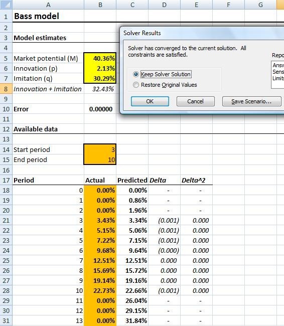
Results after running the Solver
Graph of the curve that fits the data best
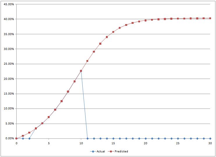
In our example, the model estimates a peak value of 40% or so. I had actually generated the series from a Bass curve, and the Solver did properly identify the value I had used to generate it. In the next installment, I will try out the model on real-world data, and test the method on the first weeks following the launch of the Chrome browser, using actual statistics from a website as a measure of its penetration, and we will see how the method holds, whether it brings any insight, and what problems we may encounter…