Gradient Boosting using Automatic Differentiation

Today, we’ll close our exploration of Gradient Boosting. First, we looked into a simplified form of the approach, and saw how to combine weak learners into a decent predictor. Then, we implemented a very basic regression tree. Today, we will put all of this together. Instead of stumps, we will progressively fit regression trees to the residuals left by our previous model; and rather than using plain residuals, we will leverage DiffSharp, an F# automatic differentiation library, to generalize the approach to arbitrary loss functions.

I won’t go back over the whole setup again here; instead I will just recap what we have at our disposition so far. Our goal is to predict the quality of a bottle of wine, based on some of its chemical characteristics, using the Wine Quality dataset from the UCI Machine Learning repository. (References: P. Cortez, A. Cerdeira, F. Almeida, T. Matos and J. Reis. Modeling wine preferences by data mining from physicochemical properties. In Decision Support Systems, Elsevier, 47(4):547-553, 2009.)

Gist available here

We are using a couple of types to model our problem:

type Wine = CsvProvider<"data/winequality-red.csv",";",InferRows=1500>

type Observation = Wine.Row
type Feature = Observation -> float
type Example = Observation * float
type Predictor = Observation -> float

To predict wine quality, we extracted 10 features from the dataset:

let features = [
    ``Alcohol Level``
    ``Chlorides``
    ``Citric Acid``
    ``Density``
    ``Fixed Acidity``
    ``Free Sulfur Dioxide``
    ``PH``
    ``Residual Sugar``
    ``Total Sulfur Dioxide``
    ``Volatile Acidity``
]

We have available a basic regression tree implementation, learnTree, which, given a sample, a list of Feature, will learn a tree to a given depth.

Using Trees instead of Stumps

Our goal now is to revisit our initial simplified boosting implementation, but use a regression tree instead of stumps. In other words, in the original version, at each iteration, we were trying to find the stump that fitted the residuals best; now we want to find the tree that fits the residuals best.

The problem statement suggests an obvious direction: we don’t really care what approach we are using, we simply want to learn the best possibly predictor given a sample. It could be stumps, or trees, or whatever you fancy. Let’s create a type to represent that:

type Learner = Example seq -> Predictor

Given a set of examples, that is, observations, and the value to predict, a Learner will do its magic, and return to us the best Predictor it can find.

All we need to do then is rearrange a bit our original code, and inject an arbitrary Learner:

let learn (sample:Example seq) (learner:Learner) (depth:int) =

    let rec next iterationsLeft predictor =
        
        // we have reached depth 0: we are done
        if iterationsLeft = 0 
        then predictor
        else
            // compute new residuals,
            let newSample = 
                sample 
                |> Seq.map (fun (obs,y) -> obs, y - predictor obs)

            // learn a predictor against residuals,
            let newPredictor = learner newSample

            // create new predictor
            let newPredictor = fun obs -> predictor obs + newPredictor obs

            // ... and keep going
            next (iterationsLeft - 1) newPredictor

    // initialize with a predictor that 
    // predicts the average sample value
    let baseValue = sample |> Seq.map snd |> Seq.average
    let basePredictor = fun (obs:Observation) -> baseValue

    next depth basePredictor

That’s pretty much it. If we want to learn a Tree, the only thing we need is to create a function with the appropriate signature; given that the trees appeared to overfit after depth 3, that’s the limit we will give them:

let treeLearner (sample:Example seq) = 
    learnTree (evenSplitter 5,sumOfSquaresCost) sample features 3
    |> predict

The treeLearner function has signature sample:seq<Example> -> (Observation -> float), so all we need to do now is to “inject” it into our learn function.

[ 1 .. 5 ]
|> List.map (fun depth ->
    let model = learn redSample treeLearner depth
    depth, averageSquareError redSample model)

In this case, we run our learning procedure at deeper and deeper levels, recording the depth and prediction quality at each step:

val it : (int * float) list =
  [(1, 0.472892841); (2, 0.4591086941); (3, 0.4564827282); (4, 0.4553268525);
   (5, 0.4550962347)]

The results are not amazing, but that’s OK, our goal here is not to create the best model for that particular problem. We just want to confirm that things are working, and this appears to be the case: as we increase depth, the average prediction error does go down.

Pseudo-Residuals and Gradients

You might have wondered by now “why is this called Gradient Boosting”? So far, there hasn’t been a single reference to a gradient. Where does this fit in?

Note that at each step of the algorithm, we are fitting a predictor to the residuals left by the current best predictor. In other words, for observation i, with a current best predictor $ F(x) $, we are computing residuals $ r_i $ as

This makes sense on an intuitive level: we are trying to learn a new model that will adjust for whatever our current best predictor “misses”. However, there is another way to look at this. If you consider the loss function:

… then the residuals as we are computing them happen to be the gradient of that particular loss function.

This is interesting, for 2 reasons. First, this connects gradient boosting to gradient descent: what we have been doing so far can be seen as gradient descent, implicitly using the sum-of-square residuals (or SSR), as a loss function, and trying at each step to find a predictor that most closely matches the gradient. Then, this allows us to generalize our algorithm. Rather than using the “plain residuals”, we can decide on any arbitrary loss function, and compute the pseudo residuals at each step as the gradient of the loss function we are interested in.

This also opens a new problem: if we do not use the SSR as a loss function, simply stacking up the predictors we get at each iteration will not necessarily give us the smallest overall loss. So instead of building our aggregate predictor as

where $ F_m(x) $ is our best predictor at stage m and $ h_m(x) $ is the predictor we fitted against the residuals, we need to now construct,

… where $ \gamma $ is the value that minimizes the loss function for $ F_m(x) $.

Replacing residuals by pseudo-residuals

Let’s leave it at that for theory, and see if we can get this to work. As a first step, we will stick with SSR as a loss function, so that we can ignore “the gamma problem”, and simply use our current algorithm, replacing the manual residuals computation by using the gradient.

Fortunately, the gradient computation is a simple problem to solve here, thanks to an awesome F# library, DiffSharp. In a nutshell, DiffSharp will take any F# function, and automatically differentiate it for you.

For simplicity, I used version 0.6.3 of DiffSharp here (by setting up the Paket dependenty to nuget diffsharp < 0.7.0). Versions 0.7 and higher support BLAS/LAPACK, which yields better performance, but is potentially more complicated. I went for ease.

Let’s add a reference to DiffSharp to our script first:

#r "fsalg/lib/fsalg.dll"
#r "diffsharp/lib/diffsharp.dll"
open DiffSharp.Numerical

What does this buy us? Let’s define a Loss type to represent a loss function:

type Loss = float -> float

The Loss will take as an input y - predictor x, and return the corresponding loss / penalty. For instance, we can define

let squareLoss : Loss = fun x -> 0.5 * pown x 2

The beauty of DiffSharp is that I can take that function, and differentiate it:

let diffSquareLoss = diff squareLoss

>
val diffSquareLoss : (float -> float)

I immediately get back a function, which I can plot:

[ - 5.0 .. 0.1 .. 5.0 ]
|> List.map (fun x -> x, diffSquareLoss x)
|> Chart.Line 
|> Chart.Show

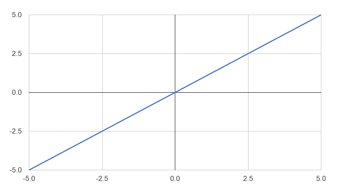
This is not the most thrilling chart, but proves our point. If we were to use squareLoss as a Loss function, then differentiating it gives us back the residuals themselves. All we have to do then is to replace our manual residuals computation, by injecting a Cost function and computing the pseudo-residuals using DiffSharp:

type Loss = float -> float

let draftBoostedLearn (sample:Example seq) (learner:Learner) (loss:Loss) (depth:int) =

    let pseudoResiduals = diff loss

    let rec next iterationsLeft predictor =
        
        // we have reached depth 0: we are done
        if iterationsLeft = 0 
        then predictor
        else
            // compute new residuals,
            let newSample = 
                sample 
                |> Seq.map (fun (obs,y) -> 
                    obs, 
                    pseudoResiduals (y - predictor obs))

            // learn a tree against residuals,
            let residualsPredictor = learner newSample

            // create new predictor
            let newPredictor = 
                fun obs -> 
                    predictor obs + residualsPredictor obs

            // ... and keep going
            next (iterationsLeft - 1) newPredictor

    // initialize with a predictor that 
    // predicts the average sample value
    let baseValue = sample |> Seq.map snd |> Seq.average
    let basePredictor = fun (obs:Observation) -> baseValue

    next depth basePredictor

If we pass in the squareLoss function, we should get exactly the same results as before. Let’s confirm this:

let squareLoss : Loss = fun x -> 0.5 * pown x 2

[ 1 .. 5 ]
|> List.map (fun depth ->
    let model = draftBoostedLearn redSample treeLearner squareLoss depth
    depth, averageSquareError redSample model)

The evaluation of our model at various depths is identical to what we had previously - it looks like we are in business:

> 
val it : (int * float) list =
  [(1, 0.472892841); (2, 0.4591086941); (3, 0.4564827282); (4, 0.4553268525);
   (5, 0.4550962347)]

Optimal model combination

Let’s tackle now the problem of finding the “right” value gamma to combine our predictors. What we want is the following: given 2 predictors f1 and f2 and a Loss function, we need to find a value gamma, such that f1 + gamma * f2 minimizes the value of the loss, summed across a sample.

Let’s start with the easy one: combining predictors. That’s straightforward:

let combination f1 f2 gamma : Predictor =
    fun obs -> f1 obs + gamma * f2 obs

If f1 and f2 are given, combination is simply a function of gamma. What we need is an algorithm that will find a value of gamma that minimizes Loss. Let’s use a slightly simplified version of the gradient descent implementation provided on the DiffSharp page:

let gradientDescent f x0 eta epsilon =
    let rec desc x =
        let g = diff f x
        if abs g < epsilon
        then x
        else
            desc (x - eta * g)
    desc x0

Explaining gradient descent would take us a bit more time than we want to spend here; in a nutshell, the algorithm takes a function and, starting from an initial value, follows the direction of steepest descent, given by the gradient. The step size is given by the parameter eta, and, once the changes become small and fall under a given threshold value epsilon, the algorithm stops.

The nice thing here is that, thanks to DiffSharp, we have a generic algorithm that will identify the minimum value for any function. As an example of usage,

let foo x = pown x 2
let min_foo = gradientDescent foo 10. 0.1 0.0001

… will find the minimum 0.0 of $ f(x) = x^2 $ , starting from x = 10.0.

All we need to do then is to use gradient descent to find the “best gamma”:

let optimalGamma (sample:Example seq) f1 f2 (penalty:Loss) =

    let combine gamma = combination f1 f2 gamma
    let costOf gamma =
        sample
        |> Seq.sumBy (fun (obs,y) ->
            combine gamma obs - y |> penalty)

    gradientDescent costOf 1.0 0.001 0.01

We create a combine function, with a single argument gamma, and a costOf function that computes, for a given value of gamma, the total cost (as measured by the loss function) summed across the sample. We can then pass that function costOf to our gradient descent implementation - if everything goes according to plan, this will spit out the optimal value of gamma.

I set the values for eta and epsilon to 0.001 and 0.01 quite arbitrarily here. Poorly chosen values for eta can cause issues: if it is too large, gradient descent will not converge. I simply tuned it by hand to work on my example - be warned that if you want to use this code, you may have to adjust it!

Let’s re-arrange again our learning algorithm, and incorporate that bit:

let boostedLearn (sample:Example seq) (learner:Learner) (loss:Loss) (depth:int) =

    let pseudoResiduals = diff loss

    let rec next iterationsLeft predictor =
        
        // we have reached depth 0: we are done
        if iterationsLeft = 0 
        then predictor
        else
            // compute new residuals,
            let newSample = 
                sample 
                |> Seq.map (fun (obs,y) -> 
                    obs, 
                    pseudoResiduals (y - predictor obs))

            // learn a tree against residuals,
            let residualsPredictor = learner newSample

            // find optimal gamma
            let gamma = optimalGamma sample predictor residualsPredictor loss

            // create new predictor
            let newPredictor =
                fun obs -> 
                    predictor obs + gamma * residualsPredictor obs

            // ... and keep going
            next (iterationsLeft - 1) newPredictor

    // initialize with a predictor that 
    // predicts the average sample value
    let baseValue = sample |> Seq.map snd |> Seq.average
    let basePredictor = fun (obs:Observation) -> baseValue

    next depth basePredictor

If everything is working as we expect, nothing should have changed. Let’s confirm that:

[ 1 .. 5 ]
|> List.map (fun depth ->
    let model = boostedLearn redSample treeLearner squareLoss depth
    depth, averageSquareError redSample model)

> 
val it : (int * float) list =
  [(1, 0.472892841); (2, 0.4591086941); (3, 0.4564827282); (4, 0.4553268525);
   (5, 0.4550962347)]

Example using the Huber loss function

So what did we gain here? So far, nothing: the net result is an added dependency, and a slower and more complex algorithm.

Stated that way, this might not appear as a great success. However, we now have the ability to plug in virtually any loss function we want.

Why would you want to do that? Using the sum-of-squares as a loss function has its benefits, but it won’t always be what you want. One of its drawbacks is that it penalizes very heavily outliers. If you have a couple of observations in your sample which your model struggles to predict, and cause large errors, using SSR as a loss function will put a very large penalty on these, and will try its best to reduce the error, at the expense of the overall sample.

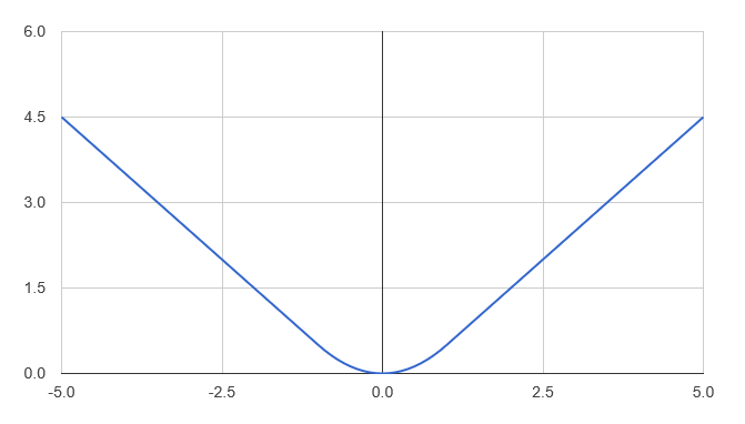
That is one reason why it is sometimes convenient to use different loss functions. As an example, let’s consider the Huber loss function (thanks @evelgab for the pointer!):

In a nutshell, what this function does is the following: for errors under a certain level delta, it applies a square penalty; beyond that level, the penalty becomes linear. In other words, small errors will get the same penalty as with the SSR, but after a certain point, the cost stops growing as aggressively. As a result, large outliers will not get slammed as hard as with SSR.

Let’s implement that function in F#:

let huber delta x = 
    if abs x <= delta
    then 0.5 * pown x 2
    else delta * (abs x - 0.5 * delta)

… and take a look at its profile:

[ - 5.0 .. 0.1 .. 5.0 ]
|> List.map (fun x -> x, huber 1.0 x)
|> Chart.Line 
|> Chart.Show

Another angle on the Huber function, perhaps more intuitive, is to consider what the pseudo-residuals would look like under Huber loss. Taking a value of 1.0 for delta, this is what we get:

let diffHuber = diff (huber 1.0)

[ - 5.0 .. 0.1 .. 5.0 ]
|> List.map (fun x -> x, diffHuber x)
|> Chart.Line 
|> Chart.Show

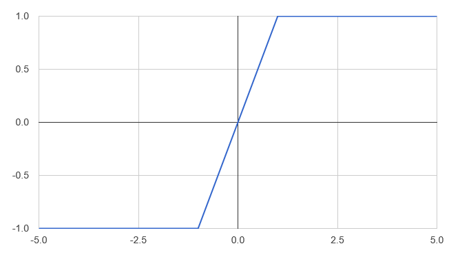
What this chart shows is that when errors go beyond +/- 1.0 the pseudo residuals flattens out. As a result, when we try to fit a predictor to the pseudo-residuals, it will treat large and very large prediction errors as equivalent.

This loss function is much more complex than the SSR. And yet, all we had to do is to write it, and DiffSharp differentiated it without blinking. We can take that function, pass it to our learning algorithm, and let diffSharp handle the differentiation work:

let huber delta x = 
    if abs x <= delta
    then 0.5 * pown x 2
    else delta * (abs x - 0.5 * delta)

let huberPredictor = boostedLearn redSample treeLearner (huber 1.0) 5

And… that’s it - it just works. No need to change anything, the algorithm will now use that loss function to compute the pseudo-residuals and gammas, all by itself.

Conclusion

That concludes our exploration of gradient boosting.

First, I want to state that the code presented here is far from optimal. Zero consideration has been given to performance, gradient descent might violently diverge, and it’s quite plausible that bugs are present. In other words, you’ve been warned, use this for inspiration, and not in production :)

My objective here was purely to explore Gradient Boosting, building the algorithm from the ground up to better understand how it works. I am glad I did; first, I find the algorithm quite interesting. It is both quite general, and fairly simple conceptually: fit your model, look at what the model didn’t catch (the residuals), try to fit another model to that, and combine the models together. I also found the idea of looking at the residuals in terms of gradient very insightful - definitely an a-ha moment.

The other interesting part to me was DiffSharp. I had spent some time with the library in the past, but hadn’t quite realized how flexible it is. When I first started writing this post, I initially used the pseudo-Huber loss function, because I assumed DiffSharp would need a continuous function to work with. I was quite surprised when, “just for fun”, I tried to differentiate the regular version I had written in plain F#, and it just worked. I guess the moral of the story is, make sure to do things “just for fun” with code - there is something waiting to be learnt there!

That’s it for me - I hope you got something out of the exercise, too!

Gist available here