Breaking down the Nelder Mead algorithm

31 Mar 2022

The Nelder-Mead algorithm is a classic numerical method for function minimization. The goal of function minimization is to find parameter values that minimize the value of some function. That description might sound abstract, but it deals with a very practical and common problem. For the Excel fans out there, the Goal Seek function is a concrete example of what function minimization is about. You want Excel to find values that make another cell equal to some value. This is a minimization problem: you are trying to make the difference between the calculated value and the target value as small as possible, by tweaking some input values.

That problem arises in many places. Regression (find parameters of a prediction function to minimize the overall prediction error), hyper-parameters optimization in machine learning, the list goes on and on.

Unfortunately, there isn’t a universal method to solve the problem. Nelder Mead is one method, and a classic (1965!). One interesting aspect of the method is that it does not rely on gradients / derivatives, but uses a heuristic that compares the value of the function at different points (the “simplex”), and progressively moves towards improvements.

It is also a method I never had a chance to really dig into, so today I figured I would break down the algorithm to figure out how it actually works. So let’s dive in!

The idea behind Nelder Mead

Note: This is my understanding of the algorithm, based on walking through this outline, and implementing accordingly. There might be errors, please let me know if you find any!

Nelder Mead starts with a collection of candidate values, the Simplex. In the example below, we have a simplex with 3 points, and we are trying to find a new point that is lower on the curve. We can compute the value of our function at each of these 3 points, and as a result we have a best current point, a worst current point, and a second-worst point.

Initial simplex

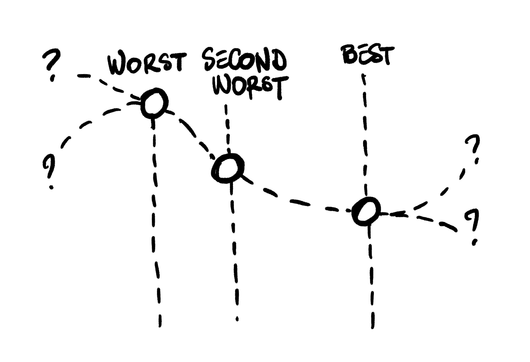
Note: the 3 points do not have to be ordered the way they are on the picture above. The worst point could be the candidate in the middle, or on the right.

Note: the algorithm also works with functions that take any number of arguments. I focused on a function with a single argument as an example here, because I found it made it easier to follow graphically what each of the steps was attempting to do.

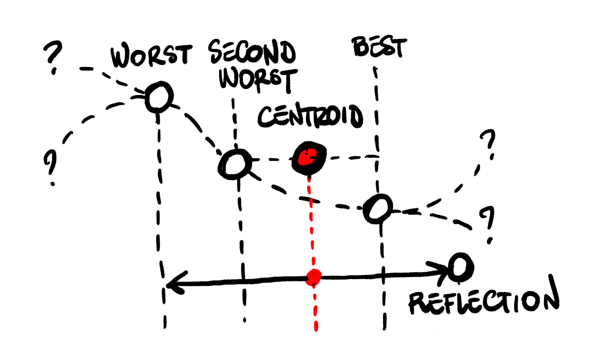
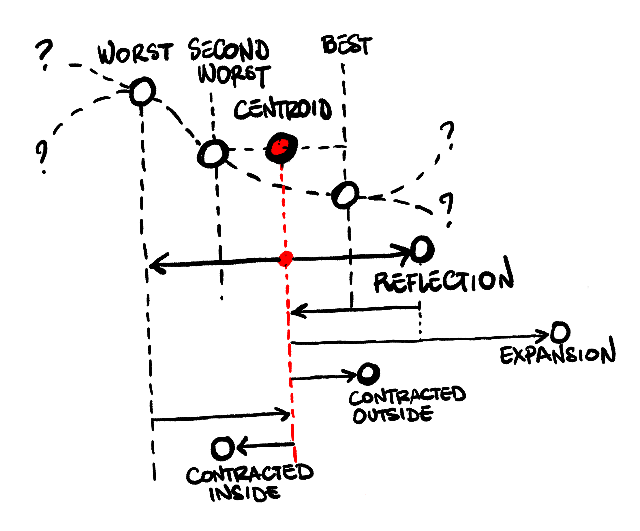
Each iteration, the algorithm will attempts to move the position of the current worst candidate. The movement will be relative to the Centroid of the remaining simplex, that is, the “center of gravity” of the other candidates. To decide what movement to take, the algorithm performs some tests:

Reflection: First, we try to move the worst candidate to the other side of the centroid. We compute the reflected candidate, a position that mirrors our worst candidate across the centroid. if that is better than our second worst candidate, but not better than the best candidate, we have a decent improvement: we simply replace our worst, and repeat.

Initial simplex

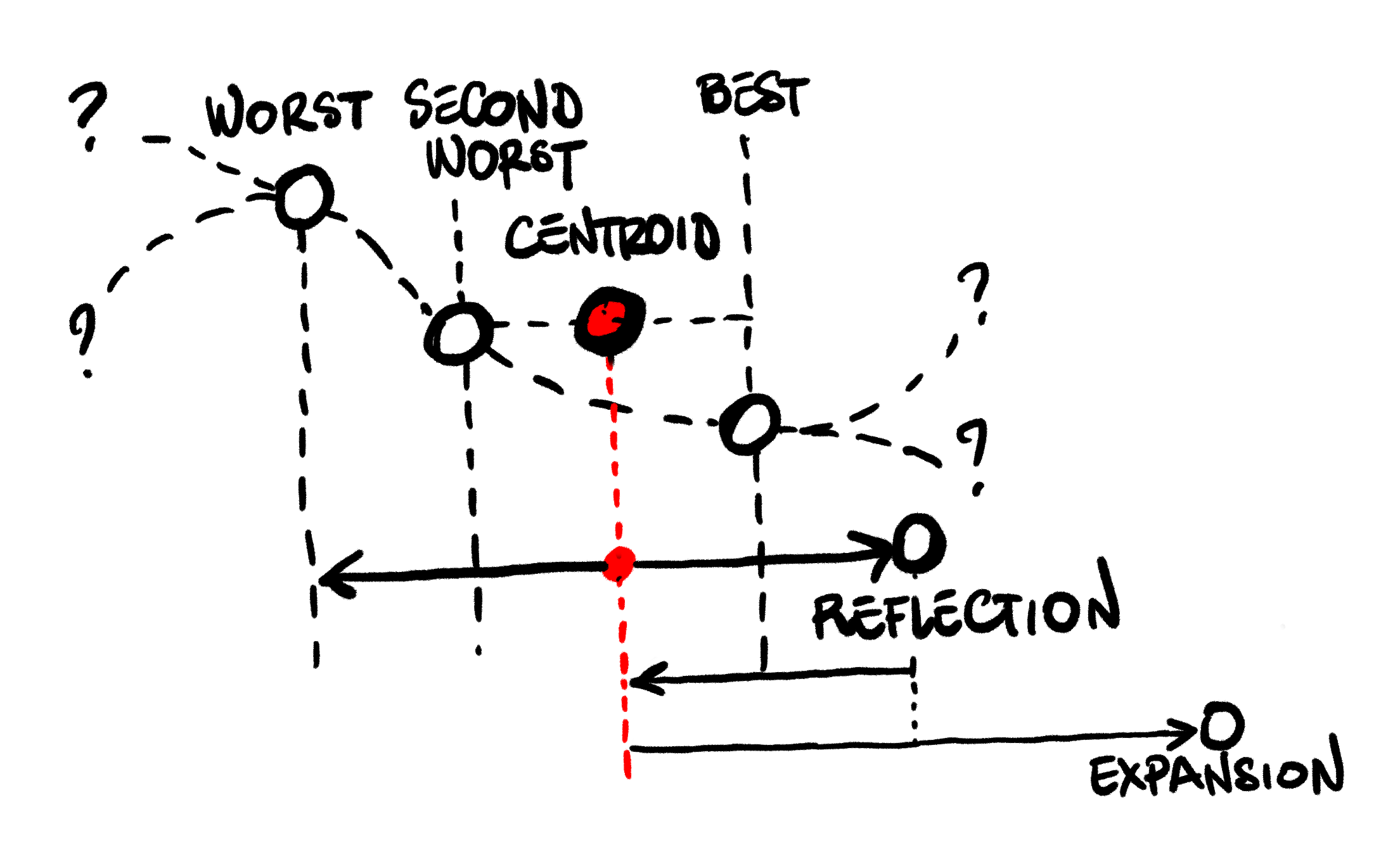
Expansion: If the reflected candidate is even better than our current best, this is a promising direction. We try to push even further in the same direction, and compute an expanded candidate. If the expanded candidate is even better, we take it and replace our current worst, otherwise we replace it with the reflected candidate, and repeat.

Initial simplex

If the reflected candidate is better than our current worst, but not better than our second worst, this is still a promising direction. We try a shorter move in the same direction: instead of expanding, we compute a contracted outside candidate, moving less aggressively towards the reflected direction. If that is better than the reflected candidate, we use it and repeat:

Initial simplex

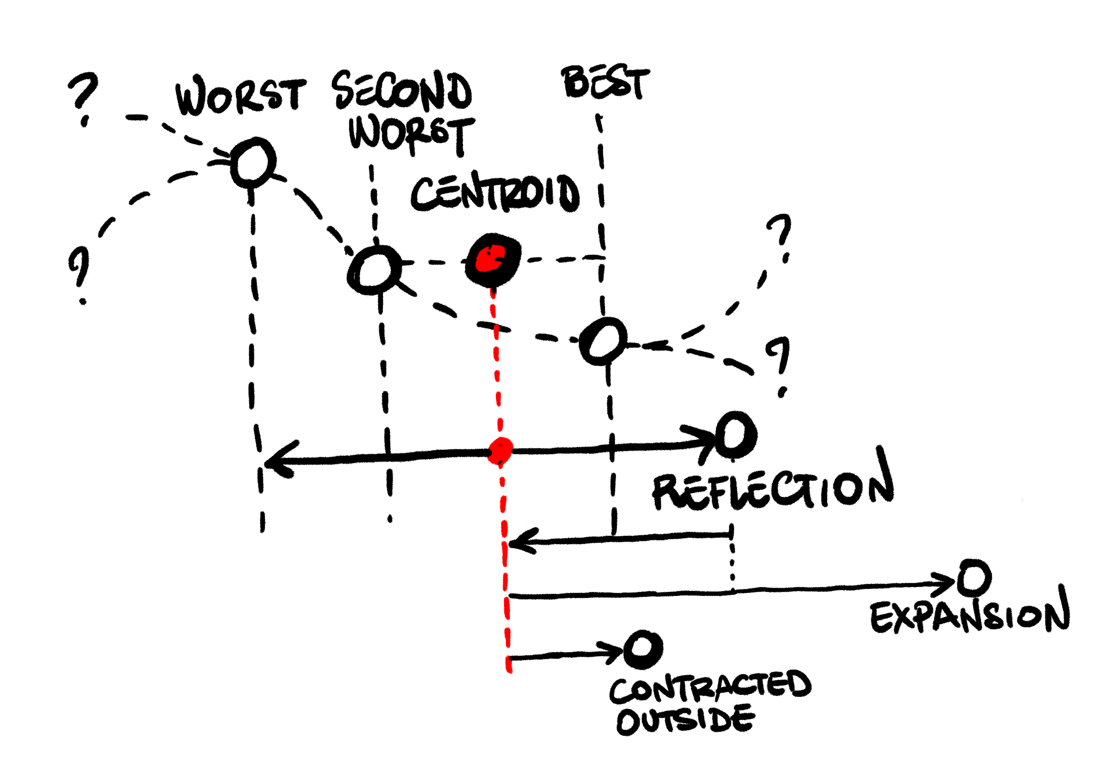
If it is not an improvement, moving towards the reflected direction does not help. Instead, we shrink: we take the whole simplex, and move every point towards the current best candidate.

Finally, if the reflected candidate is even worse than our current worst, then we attempt a move in the opposite direction, and compute a contracted inside candidate. If that is an improvement over our current worst, we take it. Otherwise, we have no good move available, and shrink the simplex:

Initial simplex

So, as I understand it, the algorithm does not directly search for a direct improvement of the candidate, like gradient descent. Instead, it searches for a promising area for an improvement, and updates the search area, moving the worst corner / edge of the simplex iteratively, taking large steps into a promising direction when it finds one, and otherwise shrinking the search area.

Which leads us to termination: when do you stop? In the version I looked at, the algorithm stops when all candidates in the simplex have values close to each other. This would happen if the search area was close to a minimum: in that case, we would expect a flat surface at the bottom of a valley, so to speak.

A rough implementation of Nelder Mead

Now that we took a look at the logic behind the algorithm… does it actually work?

To check that, we need an implementation. I took a stab at it, paying no attention to performance or style. My goal here was clarity, to make sure I understood what was going on first. There are a lot of low-hanging fruits to make the code better, I’ll revisit that later.

Without further due, here is my first take at the algorithm. The update function takes 2 arguments:

the function f that we are trying to minimize, with the expected inputs dimension dim, that is, the number of arguments it expects,
the current simplex, an array of array of floats, our current candidates.

update will take the current state of the simplex, and return an updated simplex, where the worst candidate will have been modified according to the rules described before, or the entire simplex will have been shrunk.

Note that I represented the function as float [] -> float. The float [] are the function arguments: I went for an array, because I wanted to handle functions that could take more than one argument. As an illustration, a function that adds 2 numbers would be expressed as:

let add (xs: float []) = x[0] + x[1]

Anyways, here we go: Nelder Mead update, take one:

let update (dim: int, f: float [] -> float) (simplex: (float []) []) =

    // 1) order the values, from best to worst
    let ordered =
        simplex
        |> Array.sortBy f

    // 2) calculate centroid
    let size = simplex.Length
    // drop the worst candidate
    let bestCandidates = ordered[.. size - 2]
    // calculate average point (centroid)
    let centroid =
        Array.init dim (fun col ->
            bestCandidates
            |> Array.averageBy(fun pt -> pt[col])
            )

    // 3) reflection
    let worst = ordered[size - 1]
    let alpha = 1.0
    let reflected =
        Array.init dim (fun col ->
            centroid[col] + alpha * (centroid[col] - worst[col])
            )
    let secondWorst = ordered[size - 2]
    let best = ordered[0]
    if
        f reflected < f secondWorst
        &&
        f reflected >= f best
    then
        // replace worst by reflected
        ordered[size - 1] <- reflected
        ordered

    // 4) expansion
    elif
        f reflected < f best
    then
        let gamma = 2.0
        let expanded =
            Array.init dim (fun col ->
                centroid[col] + gamma * (reflected[col] - centroid[col])
                )
        if f expanded < f reflected
        then
            ordered[size - 1] <- expanded
        else
            ordered[size - 1] <- reflected
        ordered

    // 5) contraction
    elif f reflected < f worst
    then
        let rho = 0.5
        let contractedOutside =
            Array.init dim (fun col ->
                centroid[col] + rho * (reflected[col] - centroid[col])
                )
        if f contractedOutside < f reflected
        then
            ordered[size - 1] <- contractedOutside
            ordered
        else
        // 6) shrink
            let sigma = 0.5
            let shrunk =
                ordered
                |> Array.map (fun pt ->
                    Array.init dim (fun col ->
                        best[col] + sigma * (pt[col] - best[col])
                        )
                    )
            shrunk
    elif f reflected >= f worst
    then
        let rho = 0.5
        let contractedInside =
            Array.init dim (fun col ->
                centroid[col] + rho * (worst[col] - centroid[col])
                )
        if f contractedInside < f worst
        then
            ordered[size - 1] <- contractedInside
            ordered
        else
        // 6) shrink
            let sigma = 0.5
            let shrunk =
                ordered
                |> Array.map (fun pt ->
                    Array.init dim (fun col ->
                        best[col] + sigma * (pt[col] - best[col])
                        )
                    )
            shrunk
    // 6) shrink
    else
        failwith "All cases should have been covered"

All we need at that point is a function to handle algorithm termination, and a function to create our initial simplex. Let’s go:

let terminate (tolerance: float) (f: float [] -> float) (simplex: float [][]) =
    // We stop when for every point in the simplex,
    // the function values are all close to each other.
    let evaluations = simplex |> Seq.map f
    let min = evaluations |> Seq.min
    let max = evaluations |> Seq.max
    max - min < tolerance

Given a simplex, we extract the smallest and largest function evaluations. If these are within some bounds (the tolerance), we are done.

How about initialization? We’ll go for some fairly naive approach here: given a starting point provided by the user, we will create a bunch of candidates, varying each value of the starting point by + or - 1:

let initialize (dim: int, f: float [] -> float) (startingPoint: float []) =
    [|
        yield startingPoint
        for d in 0 .. (dim - 1) ->
            let x = startingPoint |> Array.copy
            x[d] <- startingPoint[d] + 1.0
            x
        for d in 0 .. (dim - 1) ->
            let x = startingPoint |> Array.copy
            x[d] <- startingPoint[d] - 1.0
            x
    |]

Trying it out: does it actually work?

Does this thing actually work? Let’s wrap what we have in a small function, and try it out on a couple of examples:

let solve (tolerance: float) (dim: int, f: float [] -> float) (start: float []) =
    if start.Length <> dim
    then failwith $"Invalid starting point dimension: {start.Length}, expected {dim}."
    let simplex = initialize (dim, f) start
    simplex
    |> Seq.unfold (fun simplex ->
        let updatedSimplex = update (dim, f) simplex
        let solution =
            updatedSimplex
            |> Array.map (fun pt -> pt, f pt)
            |> Array.minBy snd
        Some ((solution, updatedSimplex), updatedSimplex)
        )
    |> Seq.takeWhile (fun (solution, simplex) ->
        simplex |> terminate tolerance f |> not
        )
    |> Seq.iter (fun ((solution, evaluation), _) ->
        printfn "%A: %.4f" solution evaluation
        )

Let’s try out a few simple 1 dimension examples first.

The function f(x) = x^2 has a minimum at 0.0. Let’s set the tolerance to 0.000,001 and see what happens, starting with an initial guess of 100.0.

let tolerance = 0.000_001
solve tolerance (1, fun x -> pown x[0] 2) [| 100.0 |]

[|96.5|]: 9312.2500
[|93.25|]: 8695.5625
[|86.625|]: 7503.8906
// snipped for brevity
[|-0.0003410830395|]: 0.0000
[|0.0003086419019|]: 0.0000

In about 30 iterations, we have a good solution approximation.

Let’s try f(x) = cos(x) next, starting at 0.0:

solve tolerance (1, fun x -> cos x[0]) [| 0.0 |]

In about 30 iterations, we have a solution, 3.141963005, which is pretty close to the correct answer, Pi:

[|1.0|]: 0.5403
[|2.25|]: -0.6282
[|2.75|]: -0.9243
// snipped for brevity
[|3.141963005|]: -1.0000
[|3.141963005|]: -1.0000

Let’s test it out on something more serious, using some of the classic test functions for optimization:

let beale (v: float[]) =
    let x, y = v[0], v[1]
    pown (1.5 - x + x * y) 2
    + pown (2.25 - x + x * y * y) 2
    + pown (2.625 - x + x * y * y * y) 2

solve tolerance (2, beale) [| 0.0; 0.0 |]

The Beale function has a known minimum at (3.0, 0.5), which the algorithm finds:

[|1.5; 0.0|]: 1.8281
[|1.5; 0.0|]: 1.8281
[|1.5; 0.0|]: 1.8281
[|1.5; 0.0|]: 1.8281
[|1.5; 0.0|]: 1.8281
[|3.623046875; 0.62109375|]: 0.0337
// snipped for brevity
[|3.002150137; 0.500610984|]: 0.0000
[|3.000936994; 0.5000857414|]: 0.0000
[|2.999118655; 0.4998541196|]: 0.0000
[|2.999118655; 0.4998541196|]: 0.0000

A last one for the road, the Booth function:

let booth (v: float []) =
    let x, y = v[0], v[1]
    pown (x + 2.0 * y - 7.0) 2
    + pown (2.0 * x + y - 5.0) 2

solve tolerance (2, booth) [| 0.0; 0.0 |]

Again, we find its minimum at (1.0, 3.0) in a few iterations:

[|0.0; 2.75|]: 7.3125
[|1.5; 1.875|]: 3.0781
[|1.25; 2.8125|]: 0.1133
// snipped for brevity
[|1.000358243; 3.000211252|]: 0.0000
[|1.000757956; 2.999423248|]: 0.0000
[|0.9999284495; 3.000386917|]: 0.0000

So far, so good. On our 4 examples, the algorithm did work. Will it always work? No. The function may not have a minimum, it may not be well-behaved for every input value, it may not be smooth. It may also get stuck in a local minimum if we are unlucky with our initial starting point guess. Many things could go wrong, but still: on the limited set of examples we tried out, it behaved quite nicely.

Parting words

This is where we will stop for today!

The implementation for the algorithm is pretty naive. As I mentioned before, this is a first cut: I tried my best to focus on a direct, literal transcription of the algorithm, without making any effort at optimization or style. I will probably take a stab at improving it in a follow up post. In no particular order, here is a list of things that could be improved:

Extract the reflection parameters Alpha, Gamma, Rho, Sigma,
Turn all 4 reflections into a single function,
Avoid un-necessary function evaluations,
Try to avoid un-necessary sorting of the simplex candidates,
Try to clarify the logic, removing if branches.

The solve function should also be improved, to handle situations like:

Function with no minimum (limit number of iterations),
Functions that are not defined over all numbers.

That being said, overall, we have a decent starting point - it should make for an interesting redesign exercise!

Other than that, I was pleasantly surprised at how well the algorithm works. This is particularly interesting, because the approach is fairly simple. It does not use anything complicated mathematically: all it does is, try to take a step to improve the worst candidate, probing along that direction to figure out how big that step should be. I found the overall approach interesting too, by contrast with gradient descent: instead of trying to directly find a solution, it tries to find a search area that contains a potential solution, and progressively shrink it.

Anyways, hope you found this post interesting! Ping me on Twitter if you have comments or questions, and… happy coding!

Do you have a comment or a question?
Ping me on Mastodon!