Simulating the Wrapinator 5000

It is that time of the year again! The holidays are approaching, and the F# Advent calendar is in full swing. My contribution this year might not be for the broadest audience, sorry about that :) But if you are into F#, probability theory, and numeric optimization, this post is for you - hope you enjoy it! And big shout out to Sergey Tihon for making this happen once again.

You can find the full code for this post here on GitHub.

With the Holidays approaching, Santa Claus, CEO of the Santa Corp, was worried. In preparation for the season’s spike in activity, Santa had invested in the top-of-the-line gift wrapping machine for the Elves factory, the Wrapinator 5000. This beast of a machine has two separate feeders, one delivering Paper, the other Ribbon, allowing the elves to wrap gifts at a cadence never achieved before.

So why worry? Mister Claus, being no fool, had also invested in monitoring, and the logs for the Wrapinator 5000 showed quite a few failures. Would the gift wrapping production lines hold up during the Merry Season?

Mister Claus fiddled anxiously with his luscious beard, alone in his office. And then, being a Man of Science, he did what any self-respecting CEO would do, and decided it was time to build a simulation model of his Wrapinator 5000. With a simulation model in hand, he could analyze his Elves factory, evaluate potential alternative operating policies, and most importantly, get that peace of mind he so desperately longed for.

Simulating the Wrapinator 5000, take 1

At its core, the Wrapinator 5000 has 2 components: one that delivers Wrapping Paper, and one that delivers Ribbon. While that technological marvel delivers wrapped gifts at an amazing speed, it also crashes from time to time. Both the Paper and the Ribbon feeders over-heat sometimes, requiring costly down time to reset both components and restart the machine.

Mister Claus is quite fond of iterative design. He starts his favorite editor, and decides to start with implementing a simplified version of the Wrapinator 5000, to get a feel for the problem.

Let’s start by modeling the failure causes: each cause has a name, a time to failure (the time it takes from a cold start until it crashes), and a time to fix (how long it takes to repair it once it crashed).

type FailureCause = {
    Name: string
    TimeToFailure: Random -> TimeSpan
    TimeToFix: Random -> TimeSpan
    }

Both time to failure and time to fix are somewhat random, so we model them as functions, taking a System.Random (the built-in .NET random number generator), which we will use to generate a random duration, a System.TimeSpan.

To get warmed up a little, let’s build a simple simulation here. We have 2 causes of failure, let’s start with assuming that all times are uniformly distributed:

let causes = [|
    {
        Name = "Ribbon"
        TimeToFailure =
            fun rng -> TimeSpan.FromHours (rng.NextDouble())
        TimeToFix =
            fun rng -> TimeSpan.FromHours (rng.NextDouble())
    }
    {
        Name = "Paper"
        TimeToFailure =
            fun rng -> TimeSpan.FromHours (rng.NextDouble())
        TimeToFix =
            fun rng -> TimeSpan.FromHours (rng.NextDouble())
    }
    |]

How would we go about simulating a tape of incidents using that? First, let’s model how an Incident looks like:

type Incident = {
    Cause: int
    FailureTime: DateTime
    RestartTime: DateTime
    }

Mister Claus is a bit lazy here, and decides to just use an int to indicate what FailureCause triggered the incident, referring to its index in the causes array.

Suppose that our Wrapinator 5000 started cold, what would be the next failure? In that case, both feeders are running and will fail after their TimeToFailure elapsed, and what we will observe is the first one that fails:

let nextFailure (rng: Random) (causes: FailureCause []) =
    causes
    |> Array.mapi (fun index failure ->
        index,
        failure.TimeToFailure rng,
        failure.TimeToFix rng
        )
    |> Array.minBy (fun (_, timeToFailure, _) ->
        timeToFailure
        )

We can now simulate an infinite tape representing the incidents occurring on the Wrapinator 5000: we start at some time, until our first failure occurs. When that happens, we repair the machine, based on the component that fail, we reset the two components as “fresh”, we generate an Incident, and we restart, until another failure occurs:

let simulate (rng: Random) (failures: FailureCause []) =

    let startTime = DateTime(2022, 12, 24)

    startTime
    |> Seq.unfold (fun currentTime ->
        let failureIndex, nextFailure, timeToFix =
            nextFailure rng failures
        let failureTime = currentTime + nextFailure
        let restartTime = failureTime + timeToFix
        let incident = {
            Cause = failureIndex
            FailureTime = failureTime
            RestartTime = restartTime
            }
        Some (incident, restartTime)
        )

Let’s simulate our Wrapinator 5000, with that simplified setting:

let rng = Random 0

let tape =
    causes
    |> simulate rng

let sample =
    tape
    |> Seq.take 5
    |> Seq.iter (fun incident -> printfn "%A" incident)

… we get the following tape out:

{ Cause = 0
  FailureTime = 12/24/2022 12:43:34 AM
  RestartTime = 12/24/2022 1:32:36 AM }
{ Cause = 0
  FailureTime = 12/24/2022 1:44:58 AM
  RestartTime = 12/24/2022 2:18:30 AM }
{ Cause = 1
  FailureTime = 12/24/2022 2:36:01 AM
  RestartTime = 12/24/2022 3:04:03 AM }
{ Cause = 0
  FailureTime = 12/24/2022 3:42:01 AM
  RestartTime = 12/24/2022 4:10:11 AM }
{ Cause = 1
  FailureTime = 12/24/2022 4:50:49 AM
  RestartTime = 12/24/2022 5:09:41 AM }

Here we have it - a simulation model! With Seq.unfold, we can generate an infinite tape of incidents, using failure causes following any distribution we can think of.

Mister Claus is quite pleased with himself – This is a good start.

And then he frowns. Claus can use any distribution for a FailureCause, but… which one should he use? And then, a hint of a smile forms under that glorious snow-white moustache. The logs! He has days and days of logs of that machine running and experiencing incidents, surely, he can use that to estimate some distribution!

The Shadow of a Distribution

Before going further, Mister Claus decides to take a look at that simulated tape he just generated. Let’s plot the time between failures for Cause 0, failures caused by the Ribbon feeder.

That is not too hard. We care about how long it took between 2 failures, so we reconstruct pairs of consecutive incidents, filter it down to keep only Ribbon failures, and compute the time elapsed from the last machine restart until the failure occurred:

let sample =
    tape
    |> Seq.pairwise
    |> Seq.filter (fun (_, incident) -> incident.Cause = 0)
    |> Seq.take 1000
    |> Seq.map (fun (previousIncident, incident) ->
        (incident.FailureTime - previousIncident.RestartTime).TotalHours
        )

A picture is worth a 1000 words - let’s create a histogram, to visualize how these times are distributed, using Plotly.NET:

sample
|> Chart.Histogram
|> Chart.withTitle "Ribbon: time to failure"
|> Chart.withXAxisStyle "time (hours)"
|> Chart.withYAxisStyle "number of failures"
|> Chart.show

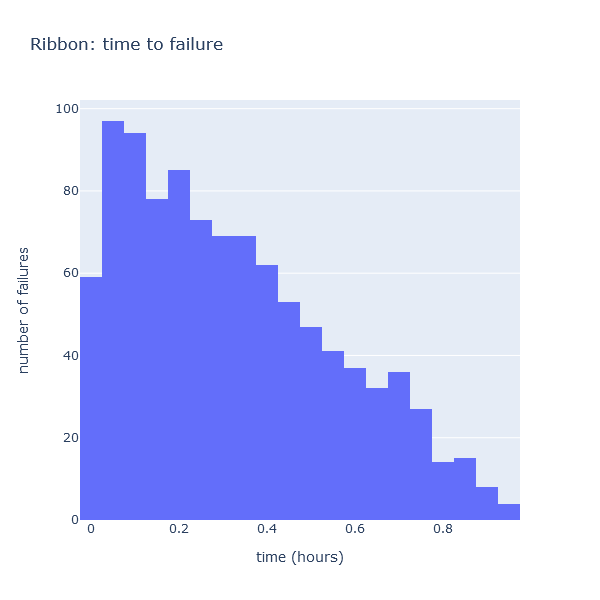
This is interesting. The Ribbon time to failure was defined as fun rng -> TimeSpan.FromHours (rng.NextDouble()): in other words, that time is uniformly distributed between 0 and 1 hours (it is equally likely to fail at any time between 0 and 1). And yet, what we observe here is most definitely not a uniform distribution, which should be flat. What is going on here?

What is going on is something a little subtle. When we observe the tape, we do not observe just the failure of the Ribbon. The 2 failures are “racing” against each other. When the Ribbon fails, we are really observing 2 things at once:

• The Ribbon Feeder failed at the time indicated,
• The Paper Feeder would have failed as well, but would have failed later.

The tape is a function of 2 distributions: each observation is the result of a race between 2 independent distributions. We see the one which happens first. Intuitively, the shape of the chart makes sense. We observe very few failures at the tail end. This is reasonable, because to observe a failure of the Ribbon Feeder that happens after, say, 0.8 hours, we need that failure to take that much time, and we also need the Paper Feeder to take even more time than the Ribbon Feeder to fail.

Note: that histogram presents another oddity. The curve looks like a triangle, except for the first bin, where we observe very few failures. I am not entirely sure what is going on there, I suspect it is a binning artifact.

Mister Claus frowns again. If the logs do not look anything like the distribution that generated each incident, how is he going to estimate these distributions?

And then a lightbulb clicks. Mister Claus remembers reading a blog post about Maximum Likelihood Estimation some time ago. Perhaps this might work! If he could express the likelihood of observing that log / tape of incidents, as a function of these failure cause distributions, then he could use Maximum Likelihood Estimation (MLE) to figure out which parameters are the most likely to have produced such a tape.

Mister Claus feels a surge of confidence. What an emotional roller coaster this is!

Simulating the Wrapinator 5000, take 2: Weibull failures

First, let’s spice up that simulation a bit, and switch from Uniform to Weibull distribution. We will keep the “why Weibull” to a minimum here; the blog post mentioned before, and the Wikipedia pages are pretty good entry points.

Weibull distributions have 2 parameters, k (the Shape parameter) and lambda (the Scale parameter). Weibulls are commonly used for time to failure in reliability models. A value of k < 1.0 describes a process that will tend to fail early (high “infant mortality”), whereas a value of k > 1.0 describes a process where as the component ages, the probability of failure keeps increasing.

Let’s implement our own Weibull:

type Weibull = {
    /// Shape parameter
    K: float
    /// Scale parameter
    Lambda: float
    }
    with
    member this.Simulate (rng: Random) =
        let p = rng.NextDouble ()
        this.Lambda * (- log (1.0 - p)) ** (1.0 / this.K)
    member this.CDF time =
        1.0
        - exp (- ((time / this.Lambda) ** this.K))
    member this.PDF time =
        (this.K / this.Lambda)
        *
        ((time / this.Lambda) ** (this.K - 1.0))
        *
        exp (- ((time / this.Lambda) ** this.K))

We represent the distribution as a record, holding the 2 parameters k and lambda, and add 3 methods, which are straight up implementations from the Wikipedia page:

• PDF, or Probability Density Function: the probability (density) to observe a failure at exactly time,
• CDF, or Cumulative Distribution Function: the probability that a failure occurred before a certain time,
• Simulate: generate a sample of that Weibull, using the Inverse Cumulative Distribution.

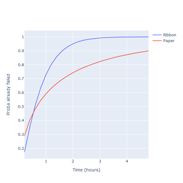
Now, we will assume that the Ribbon and Paper feeders time to failure follow a Weibull distribution, and we will pick (completely arbitrarily) parameters for these:

let weibullRibbon = {
    K = 1.2
    Lambda = 0.8
    }

let weibullPaper = {
    K = 0.6
    Lambda = 1.2
    }

Let’s plot the CDF for both of these:

let times = [ 0.2 .. 0.2 .. 5.0 ]

[
    Chart.Line (
        xy = (times |> List.map (fun t -> t, weibullRibbon.CDF t)),
        Name = "Ribbon"
        )
    Chart.Line (
        xy = (times |> List.map (fun t -> t, weibullPaper.CDF t)),
        Name = "Paper"
        )
]
|> Chart.combine
|> Chart.withXAxisStyle "Time (hours)"
|> Chart.withYAxisStyle "Proba already failed"
|> Chart.show

We can now replace our Uniform causes with Weibull distributions:

let hours = TimeSpan.FromHours

let causes = [|
    {
        Name = "Ribbon"
        TimeToFailure = weibullRibbon.Simulate >> hours
        TimeToFix = fun rng -> TimeSpan.FromHours (rng.NextDouble())
    }
    {
        Name = "Paper"
        TimeToFailure = weibullPaper.Simulate >> hours
        TimeToFix = fun rng -> TimeSpan.FromHours (rng.NextDouble())
    }
    |]

Note: we left the TimeToFix as uniform distributions, because our focus will be entirely the TimeToFailure here.

And with that small change, we are ready to simulate a tape. No change in the code, we just use different distributions for the causes:

let rng = Random 0

let tape =
    causes
    |> simulate rng

let sample =
    tape
    |> Seq.take 5
    |> Seq.iter (fun incident -> printfn "%A" incident)

… and get a different tape:

{ Cause = 0
  FailureTime = 12/24/2022 12:59:33 AM
  RestartTime = 12/24/2022 1:48:35 AM }
{ Cause = 0
  FailureTime = 12/24/2022 2:02:44 AM
  RestartTime = 12/24/2022 2:36:16 AM }
{ Cause = 1
  FailureTime = 12/24/2022 2:48:30 AM
  RestartTime = 12/24/2022 3:16:32 AM }
{ Cause = 0
  FailureTime = 12/24/2022 4:04:35 AM
  RestartTime = 12/24/2022 4:32:46 AM }
{ Cause = 0
  FailureTime = 12/24/2022 5:57:41 AM
  RestartTime = 12/24/2022 6:57:25 AM }

Structurally, that tape is similar to the one we had previously. The only key difference is that the failure times are now driven by 2 different Weibull distributions.

Note that we know exactly what Weibull distributions were used to generate that tape. Mister Claus, on the other hand, does not. All he has is the tape. The question here is, using just the tape, could he reconstruct what values of k and lambda we used? Let’s dive into this, with some Maximum Likelihood fun!

Maximum Likelihood Estimation

All Mister Claus has available are logs, which look like this:

failure 1: cause, time, restart time
failure 2: cause, time, restart time
failure 3: cause, time, restart time
...

What we are after is, given that tape, can we infer what values of k and lambda are behind the distribution of time to failure for each cause. In our example, cause 0 is Ribbon failure, cause 1 is Paper failure. Because we know what values were used in the simulation, we know what the correct answer is. We would like to write some code that takes that tape as an input, and return 4 values:

For Cause 0 (the Ribbon feeder), we expect to get back k ~ 1.2 and lambda ~ 0.8:

let weibullRibbon = {
    K = 1.2
    Lambda = 0.8
    }

For Cause 1 (the Paper feeder), we expect to get back k ~ 0.6 and lambda ~ 1.2:

let weibullPaper = {
    K = 0.6
    Lambda = 1.2
    }

Let’s consider one of the failures from the tape, say:

failure 42: cause 1, failed at 16:00, fixed at 16:47

Because we are interested in the time it took for the failure to occur, we need to know when the machine last started, which is the restart time after the previous failure:

failure 41: cause 0, failed at 15:05, fixed at 15:15
failure 42: cause 1, failed at 16:00, fixed at 16:47

The time between failures is 16:00 - 15:15, that is, 45 minutes.

Now the question is, if we assume that the Ribbon and Paper time to failure each follow a Weibull distribution, what is the probability of observing that particular event in the tape?

Let’s denote these 2 distributions as

Ribbon: Weibull_0 (k_0, lambda_0)
Paper: Weibull_1 (k_1, lambda_1)

The cause of failure 42 was 1, that is, the Paper failed, after 45 minutes. For this to happen, 2 things need to be true:

• The Paper failed at exactly 45m. The probability of this event is Probability (Weibull_1) = 45 minutes, which is given by its Probability Density Function, or PDF: PDF (Weibull_1) = 45 minutes.
• The Ribbon did NOT fail before 45m. The probability of this event is Probability (Weibull_0) > 45m, which is given by 1 - its Cumulative Distribution Function, or CDF: 1.0 - CDF (Weibull_0) = 45m.

The probability of 2 independent events is their product, so the probability of observing a Paper failure occurring exactly at 45 minutes is:

(1.0 - CDF (Weibull_0)) * (PDF (Weibull_1))

Note: the same approach generalizes to more failure causes. In that case, the probability to observe a particular event is the PDF of that event, multiplied by the CDF of every event that did NOT occur.

Armed with this, we can now compute the likelihood of observing a particular event i in the tape, with a time to failure t:

$Likelihood(i,t) = PDF_i(t) \times \prod_{j \neq i}{(1-CDF_j(t))}$

Armed with this, we can now determine the likelihood of observing a particular failure in our sample. All we need to do is plug in the formula for the corresponding PFD and CDF for the Weibull distribution.

However, what we are after is the likelihood of observing the full tape we have available, given a set of values for $k_0, lambda_0$ and $k_1, lambda_1$. That is not too complicated: again, assuming observations are independent, the probability of observing the whole tape is the product of the probabilities of observing each individual event.

In other words, if we have a tape like this one:

observation_1: cause_1 = 0, time_1 = 25
observation_2: cause_2 = 1, time_2 = 48
observation_3: cause_3 = 0, time_3 = 43
etc ...
observation_n: cause_n = 0, time_n = 27

Then the likelihood of observing that tape (given $k_0, lambda_0$ and $k_1, lambda_1$) will be

$Likelihood(tape)=Likelihood(observation_1) \times Likelihood(observation_2) \times … \times Likelihood(observation_n)$

The beauty here is that we have now a function, the Likelihood, which allows us to quantify how likely it is that a particular set of values $k_0, lambda_0$ and $k_1, lambda_1$ would have generated a particular tape. This is great, because we can use the likelihood function to answer the following question: what are the 4 values of $k_0, lambda_0$ and $k_1, lambda_1$ that are the most likely to have generated the tape we are observing. In other words, if we can find the 4 values that maximize the likelihood function, we will have solid estimates for our 2 Weibull distributions.

Before going further, let’s make that problem a bit easier to work with. First, we can use the classic log-likelihood “trick”, and convert this expression into a log likelihood:

$ln(Likelihood(tape)) = ln(Likelihood(observation_1)) + … + ln(Likelihood(observation_n))$

This is useful, because this function will reach its maximum for the same arguments, but we are now dealing with a sum instead of a product.

Let’s dig a bit deeper here, and inspect $ln(Likelihood(observation))$:

$ln(Likelihood(observation=i,t))=ln(PDF_i(t) * \prod_{j \neq i}{(1-CDF_j(t))})$

Again, we are dealing with a product, and because $ln(a \times b)=ln(a)+ln(b)$, we can transform this into a sum:

$ln(Likelihood(observation=i,t))=ln(PDF_i(t)) + \sum_{j \neq i}{ln(1-CDF_j(t))})$

Why do we care? We care, because this makes our maximization problem separable. If we consider for instance $k_0, lambda_0$, these 2 arguments will appear only in one PDF or CDF term, and the rest of the expression will be a constant with respect to $k_0, lambda_0$.

Practically, what this means is that we can simplify our maximization problem. Instead of maximizing one complicated function of 4 arguments $k_0, lambda_0$ and $k_1, lambda_1$, we can maximize independently 2 simpler functions, one that depends only on $k_0, lambda_0$, and one that depends only on $k_1, lambda_1$.

Likelihood Surface

Before attacking the maximization itself, let’s take a step back from math and revert to F# code for a little, to illustrate what is happening in code, rather than in equations.

Fundamentally, what the last point means is that for each FailureCause, we can take their parameters k and lambda, and estimate the likelihood of having generated the tape we observe.

In the end, the likelihood function boils down to this. In the tape, if we observe the cause we care about, use the PDF, otherwise, use (1 - CDF). We can prepare our tape of Incident(s) for the cause we care about, extracting the time between failures, and flagging with a boolean whether or not the cause we observe is the one we care about:

let prepare (index: int) (tape: Incident []) =
    tape
    |> Array.pairwise
    |> Array.map (fun (previousIncident, incident) ->
        incident.Cause = index,
        (incident.FailureTime - previousIncident.RestartTime).TotalHours
        )

The boolean here indicates essentially whether or not the cause we care about “won” the race, and occurred first. If it did, we want to use the PDF, otherwise, we use (1 - CDF). This results in the following function, the likelihood that 2 values (k, lambda) were the ones generating our tape:

let likelihood (k, lambda) (sample: (bool * float) []) =
    let weibull = { K = k; Lambda = lambda }
    sample
    |> Array.sumBy (fun (observed, time) ->
        if observed
        then weibull.PDF time |> log
        else (1.0 - weibull.CDF time) |> log
        )

In theory, out of the infinitely many possible pairs of values (k, lambda), one of them will give us a maximum value. That pair is the one that is the most likely to have generated the sample, and, as a result, it should also be close to the actual value we used to simulate that sample.

Let’s see if that actually works, by plotting the likelihood as a Plotly surface for a range of values of k and lambda, essentially doing a visual grid search:

let ribbonSample =
    sample
    |> Estimation.prepare 0
    |> Array.truncate 100

let ks = [ 0.5 .. 0.05 .. 2.0 ]
let lambdas = [ 0.5 .. 0.05 .. 2.0 ]

let z =
    [
        for k in ks ->
            [ for lambda in lambdas -> likelihood (k, lambda) ribbonSample ]
    ]

Chart.Surface (
    z,
    X = ks,
    Y = lambdas,
    Contours = TraceObjects.Contours.initXyz(Show = true)
    )
|> Chart.withTitle "Ribbon: log likelihood"
|> Chart.withXAxisStyle ("k", Id = StyleParam.SubPlotId.Scene 1)
|> Chart.withYAxisStyle ("lambda", Id = StyleParam.SubPlotId.Scene 1)
|> Chart.withZAxisStyle "log likelihood"
|> Chart.show

The resulting chart displays, for values of k and lambda between 0.5 and 2.0, what the log likelihood is. The higher the “altitude”, the more likely it is that the corresponding pair of coordinates generated the sample tape:

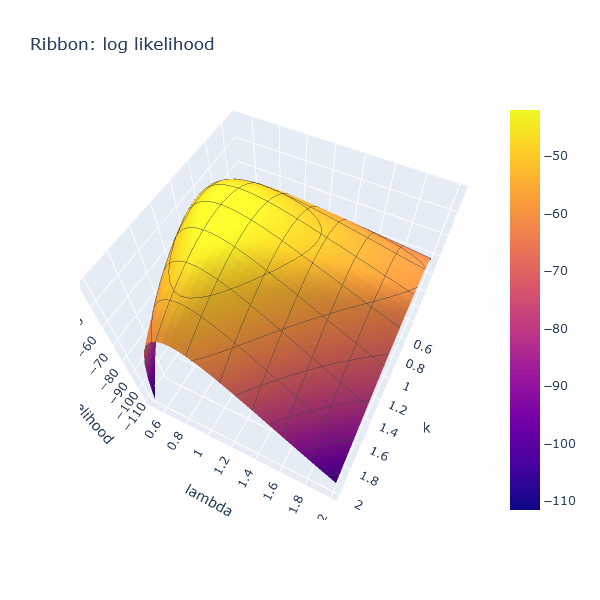
That surface is convex, and forms a nice hill, with a peak in roughly the correct area, around k ~ 1.3, lambda ~ 0.8.

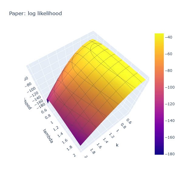
Similarly, we can plot the log likelihood for Paper, which also produces a convex hill, with a peak at a different position.

First, this confirms that the idea has legs. Then, from a numeric optimization standpoint, this is good news. If we have a convex surface, all we need is a hill climbing algorithm. We can start from any value of k and lambda, for instance (1.0, 1.0), and take small steps that always go uphill.

One such hill climbing algorithm is Gradient Descent, or, rather, Gradient Ascent in this case. Starting from values (k = 1.0, lambda = 1.0), compute the partial derivative of the log likelihood, and take a small step towards the direction with a positive gradient.

Let’s do this.

MLE using Gradient Ascent with DiffSharp

The tricky part here is the step “compute the partial derivative”. Manually computing the partial derivative of the log-likelihood function would be quite painful. Fortunately, thanks to DiffSharp, an F# automatic differentiation library, we can mostly ignore that issue, and let the library do the heavy lifting for us. This is what we will do here.

I won’t cover that part in detail, because I went through something similar in this post. You can find the whole code performing the MLE using gradient descent here.

How does it work when we run that code against our tape? Let’s check:

let sample =
    tape
    |> Seq.take 100
    |> Seq.toArray

let ribbon =
    sample
    |> Estimation.prepare 0
    |> Estimation.estimate

printfn "Ribbon: %A" ribbon

After some iterations, we get our estimate for what good parameters for the Ribbon failure distribution might be:

Ribbon: { K = 1.217164993
  Lambda = 0.8133975863 }

Similarly, we get the following estimates for the Paper failures:

Paper: { K = 0.6178998351
  Lambda = 1.249123335 }

The values we used to generate that tape were:

let weibullRibbon = {
    K = 1.2
    Lambda = 0.8
    }

let weibullPaper = {
    K = 0.6
    Lambda = 1.2
    }

Pretty close, I would say!

Conclusion

That is as far as we will go today!

I realize that this topic is probably a tad esoteric for most. However, I found it personally very interesting. I never really got into Maximum Likelihood Estimation techniques in the past, in large part because they involve calculus, which is something I am not good at. I find it quite impressive how, with the help of DiffSharp, it took fairly little code to make it all work.

On the probability front, I was quite surprised when I realized that the problem was separable. The result is interesting to me, for 2 reasons. First, we end up using the full tape of failures for every event. Even when we do not observe the event type we care about, we have usable information, because we know that the event in question did not “win the race”. Then, fundamentally the log likelihood for each distribution depends only on the PDF and CDF for that distribution, and nothing else. As an interesting result, the approach can be generalized to any mixture of distributions, as long as we have a PDF and CDF for it.

As a side-note, shout out to the awesome F# crew at Simulation Dynamics. Many of the ideas presented in this post emerged from discussions with them :)

Anyways, I hope that you got something out of this post. If you have questions or comments, hit me up on Twitter or Mastodon. In the meantime, have fun coding, be nice to each other, and wish you all wonderful holidays!

Full code here on GitHub