Study notes: function minimization with DiffSharp

This post is intended primarily as a note to myself, keeping track as my findings as I dig into automatic differentiation with DiffSharp. Warning: as a result, I won’t make a particular effort at pedagogy – hopefully you’ll still find something of interest in here!

The main question I am interested in here is, how can I use DiffSharp to find the minimum of a function? I will take a look first at basic gradient descent, to get us warmed up. In a future installment I plan to explore using the built-in SGD and Adam optimizers for that same task.

The full code is here on GitHub, available as a .NET interactive notebook.

Test function

The function we will be using in our exploration is the following:

$f(x,y)=0.26 \times (x^2+y^2) - 0.48 \times (x \times y)$

This function, which I lifted this function from this blog post, translates into this F# code:

let f (x: float, y: float) =
    0.26 * (pown x 2 + pown y 2) - 0.48 * x * y

Graphically, this is how the function looks like:

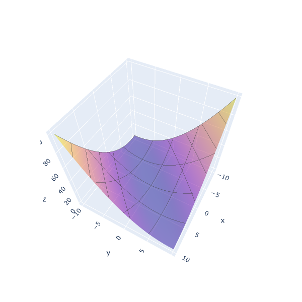
This function has a global minimum for (x = 0.0, y = 0.0), and is unimodal, that is, it has a single peak (or valley in this case). This makes it a good test candidate for function minimization using gradient descent.

To visualize the surface of a function of 2 variables, we use the following utility function:

let surface ((xMin, xMax), (yMin, yMax)) f =
    let xStep = (xMax - xMin) / 100.0
    let yStep = (yMax - yMin) / 100.0
    let xs = [| xMin .. xStep .. xMax |]
    let ys = [| yMin .. yStep .. yMax |]
    let z =
        Array.init ys.Length (fun yi ->
            Array.init xs.Length (fun xi -> f (xs.[xi], ys.[yi]))
            )
    Chart.Surface (
        z,
        X = xs,
        Y = ys,
        Opacity = 0.5,
        Contours = Contours.initXyz (Show=true),
        ShowScale = false
        )

… which we can use to plot our function f over the range x in (-10.0; 10.0) and y in (-10.0; 10.0):

f |> surface ((-10.0, 10.0), (-10.0, 10.0)) |> Chart.show

Basic Gradient Descent

The idea of Gradient Descent is simple: to minimize a function f, starting from a position x, compute the gradient of the function at x, and take a step opposite of the gradient to go downhill.

This is easy enough to express with DiffSharp. The parameter lr here is the learning rate, a positive number describing how large of a step we want to take:

let gradientStep (lr: float) x f =
    let g = dsharp.grad f x
    x - lr * g

Let’s confirm that this works on our example, which we rewrite in terms of Tensor instead of float (more on that later):

let objective (input: Tensor) =
    let x = input.[0]
    let y = input.[1]
    0.26 * (pown x 2 + pown y 2) - 0.48 * x * y

We can compute the value of our function at the point (5.0, 5.0):

objective (dsharp.tensor [ 5.0; 5.0 ]) |> float

… which produces the value 1.0000009536743164

Let’s take a gradient step, and evaluate the function again:

let updated =
    objective
    |> gradientStep 0.25 (dsharp.tensor [ 5.0; 5.0 ])
updated
|> objective
|> float

The value of the objective function at our updated position is now 0.9800996780395508, which is lower than the initial value, 1.0000009536743164. We did indeed move downhill.

Armed with this, we can write Gradient Descent as an infinite sequence of steps, repeatedly taking gradient steps and updating our position:

let gradientDescent lr init f =
    init
    |> Seq.unfold (fun x ->
        let updated = gradientStep lr x f
        let objectiveValue = f updated
        Some ((updated, objectiveValue), updated)
        )

At each step, we generate the updated position, as well as the new value of the objective function. As an example, we can view the first 5 iterations of gradient descent on f, starting at position (5.0, 5.0):

objective
|> gradientDescent 0.25 (dsharp.tensor [ 5.0; 5.0 ])
|> Seq.take 5
|> Seq.map (fun (coeffs, value) ->
    (coeffs.[0] |> float, coeffs.[1] |> float),
    value |> float
    )

(X, Y)                      Objective
(4.949999809, 4.949999809), 0.980099678
(4.900499821, 4.900499821), 0.9605951309
(4.851494789, 4.851494789), 0.9414796829
(4.802979946, 4.802979946), 0.9227437973
(4.754950047, 4.754950047), 0.904381752

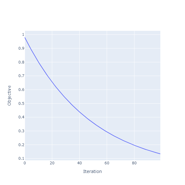
We can plot the decrease of the function over 100 iterations:

objective
|> gradientDescent 0.25 (dsharp.tensor [ 5.0; 5.0 ])
|> Seq.take 100
|> Seq.mapi (fun i (coeffs, value) -> i, float value)
|> Chart.Line
|> Chart.withXAxisStyle "Iteration"
|> Chart.withYAxisStyle "Objective"

Visualizing gradient descent on the function surface

Can we visualize how the algorithm behaves for different values of lr, the learning rate? Let’s do this. In addition to the surface itself, we need to plot the position of a sequence of coordinates over that surface.

Let’s write a function to plot such a trajectory, taking in a sequence of positions, and the function that defines the surface:

let trajectory positions f =
    let coordinates =
        positions
        |> Seq.map (fun (x, y) -> x, y, f (x, y)
        )
    Chart.Scatter3D (
        coordinates,
        mode = StyleParam.Mode.Lines_Markers,
        Marker = Marker.init(Size = 3)
        )

let named name = Chart.withTraceInfo(Name = name)

All we have to do then is create 3 sequences of gradient descent, each using a different value for lr, the learning rate, and compose them into one chart, like so:

let traj1 =
    objective
    |> gradientDescent 0.25 (dsharp.tensor [ -5.0; 10.0 ])
    |> Seq.take 1000
    |> Seq.mapi (fun i (pos, _) -> i, (pos.[0] |> float, pos.[1] |> float))
    |> Seq.filter (fun (i, pos) -> i % 1 = 0)
    |> Seq.map snd

let traj2 =
    objective
    |> gradientDescent 0.10 (dsharp.tensor [ -5.0; 10.0 ])
    |> Seq.take 1000
    |> Seq.mapi (fun i (pos, _) -> i, (pos.[0] |> float, pos.[1] |> float))
    |> Seq.filter (fun (i, pos) -> i % 1 = 0)
    |> Seq.map snd

let traj3 =
    objective
    |> gradientDescent 2.0 (dsharp.tensor [ -5.0; 10.0 ])
    |> Seq.take 100
    |> Seq.mapi (fun i (pos, _) -> i, (pos.[0] |> float, pos.[1] |> float))
    |> Seq.filter (fun (i, pos) -> i % 1 = 0)
    |> Seq.map snd    

[
    f |> surface ((-10.0, 10.0), (-10.0, 10.0))
    f |> trajectory traj1 |> named "lr = 0.25"
    f |> trajectory traj2 |> named "lr = 0.10"
    f |> trajectory traj3 |> named "lr = 2.00"
]
|> Chart.combine
|> Chart.withXAxisStyle("X", Id = StyleParam.SubPlotId.Scene 1, MinMax = (-10.0, 10.0))
|> Chart.withYAxisStyle("Y", Id = StyleParam.SubPlotId.Scene 1, MinMax = (-10.0, 10.0))
|> Chart.withZAxisStyle("Z", MinMax = (0.0, 120.0))
|> Chart.withSize (800, 800)
|> Chart.show

… which produces a chart like this one:

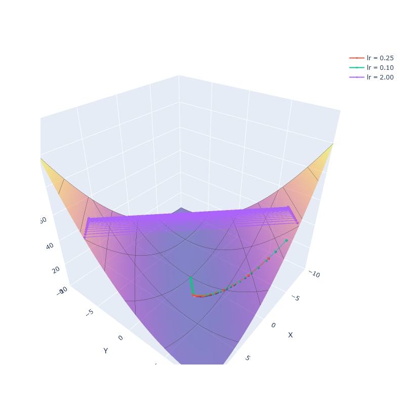
The chart highlights two interesting things:

First, the sequences generated with learning rates of 0.25 and 0.1 are very similar. They follow the same general path, first following the steepest hill down the valley, then taking a turn to follow the much gentler slope of the “inner valley”. The main difference between the two is in how quickly they progress: a learning rate of 0.25 takes larger steps each iteration, progressing faster to the minimum of the function f.

Second, the sequence generated with a learning rate of 2.0 looks quite different. Instead of descending regularly towards the minimum, it bounces back and forth between the two sides of the valley. What is happening here is, the step we are taking is too large, and we end up over-shooting beyond the point where we are descending. This is a known issue with gradient descent. We compute the gradient at our current point, which describes how the slope looks like in the immediate neighborhood of that point. The further away we go from our current point, the less likely it is that the surface there still looks the same.

Which leaves us with an annnoying quandary. In order for gradient descent to work, we need to set a learning rate, and setting that value is problematic. On the one hand, we want to take a large learning rate, so we can converge to the minimum faster. On the other hand, if we pick a learning rate that is too large, we risk not converging at all.

Parting notes

That’s where I will stop for today!

In a next installment, I plan to follow up on the same topic, trying to use the built-in Adam and SGD optimizers, instead of basic gradient descent. These two approaches build on gradient descent, adding some modifications around adapting the learning rate iteratively.

Anyways, I hope that you got something out of this post. If you have questions or comments, hit me up on Mastodon or Twitter. In the meantime, have fun coding, be nice to each other, and hope you all have a wonderful year 2023 ahead!

Full code here on GitHub