Gauging the potential of Chrome using the Bass model (part 2)

01 Oct 2008

In my previous post, I described how the Bass model can be used to forecast the market potential for a newly introduced product, using limited post-introduction data. In this post, I will apply the method to a real-world situation, to see how the method holds up in practice, what practical problems may arise, and how to address them.

The data

My objective is to evaluate the long-term share of internet traffic of Chrome, the new Google browser. I will be using actual traffic data from a medium-sized website, the technology blog of Donn Felker. In case you wonder why I didn’t use my own data, unfortunately my own traffic is not steady enough to get a “statistically decent” sample of Chrome users, and Donn was gracious enough to share his data with me (Thank you!).

The data I will be using is the percentage of visits coming from users using Chrome as a browser. It covers September 2 to September 17, 2008, the 2 first weeks of Chrome on the market.

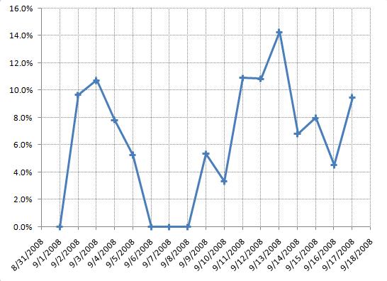
Running the fitting procedure on the raw data yields the following curve; it is clearly a (very) poor fit, which is not too surprising given the obvious discrepancy between the shape of the Bass curve and the actual data. What we are hoping for is a nice, smoothly growing, S-shaped adoption curve - and what we get is a big bump in the first few days, followed by a collapse and a “second-wind” of unsteady growth, with fluctuations up and down. It is clear right off the bat that we have a problem.

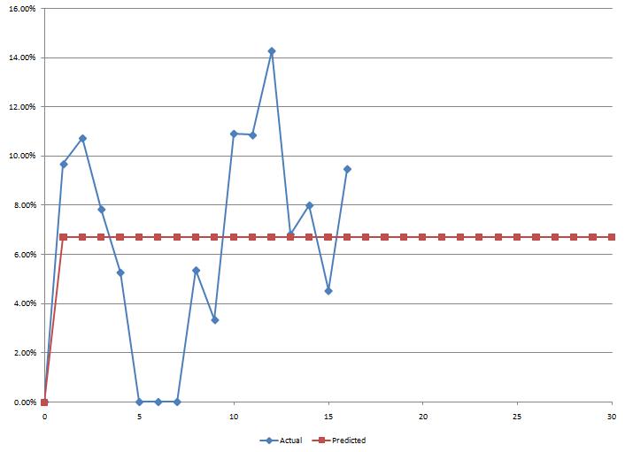
Somewhat interestingly, the model concludes that we have 100% of innovators and 0% imitators; in other words, it interprets the curve as an early adoption spike, immediately reaching its potential and fluctuating around it with “some” noise. It points at one central question we need to address: how to understand the spike and collapse of the first week?

The problem of experimenters

What is the source of the problem? My guess is that the initial spike comes from “experimenters”. When Chrome was released, I installed it and gave it a ride - and went back to Firefox, because Chrome does not support add-ons. I did not “adopt” Chrome, I just tried it out - but I would show up as an adopter on measured traffic.

The standard Bass model does not account well for this situation. The frame of the Bass model is an “irreversible” adoption: once you adopt a product, you own it. Think of buying a durable good, like a car or a fridge - you don’t try to return it to the retailer after a few days because you don’t like it.

I initially thought about two other factors. First, most websites display a seasonal pattern; typically, week-ends are “slow” (quite a few people surf from work, and do better things in their free time). Then, this website is a blog, which means that spikes of traffic are likely to be observed when a new entry is posted, as people following the feed will visit the site. However, these two factors are not directly relevant here, as we are observing the proportion of Chrome users: these would matter only if we measured absolute traffic, in number of hits.

These do have an indirect impact, however, in assessing how reliable the measurement of Chrome traffic is. In a nutshell, if in a given day there isn’t much traffic altogether, then the proportion of Chrome users I will observe is going to be less reliable than in a heavy day, because of the small size of the overall sample. I will go back to that point later.

The easiest way to get around the issue, without modifying the Bass model to account for experimenters who abandon the product midway through, is to use one of the oldest and most robust analytical devices ever , the eyeballing approach. Looking at the raw data, the first week of data visibly does not follow the pattern we expect. One possible approach is to ignore that data as initial noise, and begin the fitting after the curve has somewhat stabilized.

When running the fitting process beginning at the 5th data point, I obtain the following curve:

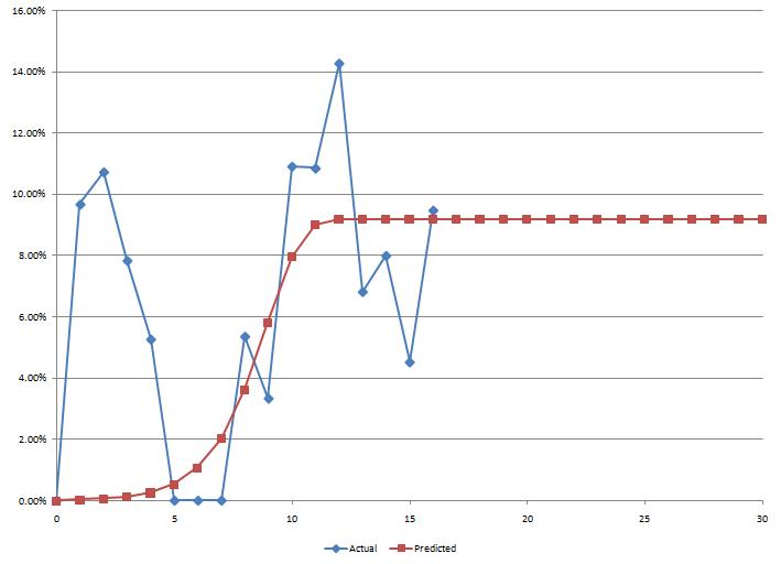
The predicted long-term usage is around 9%.

Given the available data, I think this is a reasonable estimate. However, I would certainly not bet the house on that number. The last 5 observations fluctuate between 5% and 14%, which is a huge range. Furthermore, there is no clear stabilization of the trend: each of the five last moves changes direction.

With one more week of data to confirm stabilization, I would hope to get more confidence; but as of now, the results of the model are somewhat inconclusive, and at that point, I would not trust my results to be any more reliable than the expert opinion of Donn, based on his experience and gut feeling.

Technically, there are some additional steps I could take to improve my confidence in the results. Rather than minimizing the sum of the square of the differences, I could try to minimize other fit-quality criteria, such as the mean absolute error. I could also add some weight on the observation errors, based on the size of the traffic that day. However, in my opinion, these would still not address the fundamental problem, namely, that the first week of observations does not fit the pattern we expect, and therefore, we will have to ultimately resort to human judgment - which is probably a good thing, as blind trust in the outputs of a quantitative model can lead to dramatic mistakes.

In other words, score one for humans!